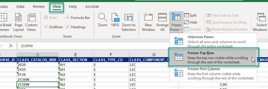
Tip #1: Freeze the Top Row to Make Scrolling More User Friendly
It is not uncommon for reports at UConn to include hundreds or even thousands of rows and dozens of columns of data. When working with datasets this large, it can be easy to lose track of the heading of each column as you scroll. To lock the heading row in place, use Freeze Top Row. Go to the View tab and expand the menu under "Freeze Panes" in the Window group, and click "Freeze Top Row":
Tip #2: Add Filter Buttons to Your Columns for Easy Filtering and Sorting
Most of the time, you will want to focus on certain subsets of data within the larger data set. You can search in Excel the same way you can in other Office programs (CTRL+F), but filtering and sorting particular columns is usually a better approach.
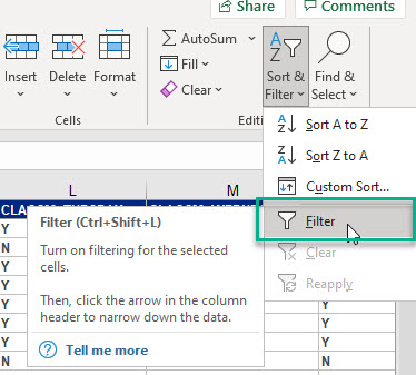
Add Filter Buttons to Each Heading
On the Home tab of the ribbon, click the "Sort & Filter" button from the Editing group and select "Filter":
Doing this will add drop-down buttons to each heading with a number of filter and sort options:
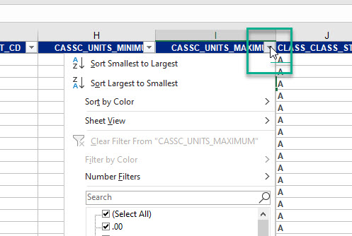
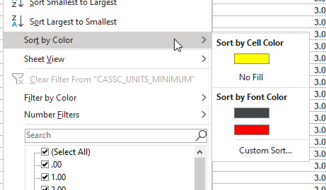
Sort Options
Sort options will vary depending on the type of field you're sorting with (e.g. "smallest to largest" for numbers, "A to Z" for text, "oldest to newest" for dates and times, etc.) and you can sort in either ascending or descending order. If you've used colors to organize your data, you can also sort by font or cell color:
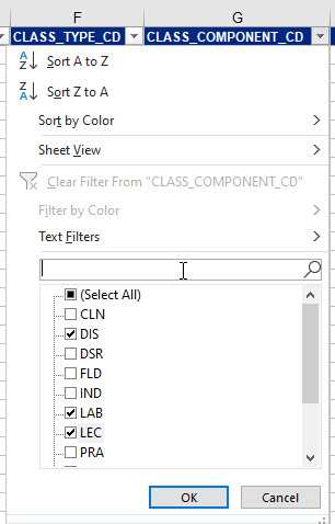
Filter Options
There are several ways to filter your results. The first is to simply check the items from the list that you wish to display by checking the box next to each item you want to see. In this example, I've selected only "DIS," "LAB," and "LEC":
All filters in Excel are progressive, meaning that as you add filters, your results for each successive filter will only be pulled from the results you have already filtered. For example, if I wanted to filter the data set to which I just added a filter to include only classes that meet on Mondays, the results I see from the second filter would also have the first filter in place, so I'd only see DIS, LAB, and LEC classes that meet on Mondays.
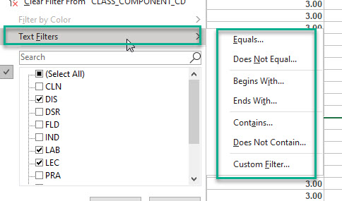
Other Ways to Filter
If you have a very large dataset and don't want to select items individually, you can filter in different ways depending on the type of data in the column you're working with. For example, when filtering text fields, you can filter based on the content of cells:
Other data types have different options. For example, you can filter number fields to show only values greater than, less than, or between values that you specify.
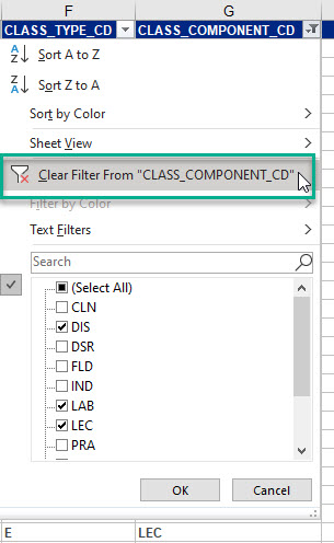
Clear Filters
You can mix and match filters as much as you want and clear filters you no longer need using the same menu on a field by field basis:
You can also clear all filters at once by clicking the same "Sort & Filter" menu you used to add the filter buttons to each heading.
Tip #3: Use Custom Sort for Multi-Level Sorting
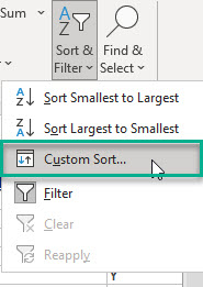
While the drop-down menu in Tip #2 makes it easy to sort your data set by a single field, sometimes you need to sort by several fields at once. To do this, use "Custom Sort" from the Sort & Filter menu:
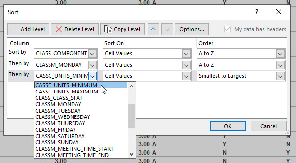
In the example below, I've set my data set to sort first by component, then by whether the class meets on Monday, and then by the minimum units:
Use sorting methods in combination with filtering to drill down even further into your data.
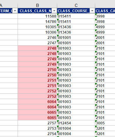
Tip #4: Use Conditional Formatting to Highlight Certain Values
Conditional Formatting allows you to highlight cells with color so that you can easily find those that fit your criteria. For example, there is a built in function that allows you to highlight duplicate values. Here's how it works.
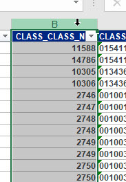
Step 1: Click the Letter Above the Heading to Select an Entire Column
Here, I've moved my cursor to the "B" above my second column and clicked it when my cursor changed to a down arrow:
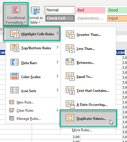
On the Home tab, go to Conditional Formatting > Highlight Cells Rules > Duplicate Values...
...and then choose the format you want to apply to the duplicate cells from either the built-in formats or your own custom format:
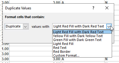
Once you make your selection, Excel will automatically change the formatting of all duplicate cells: